15. Other Classic ML Models (2)

Support Vector Machines

Support Vector Machines (SVMs)

2000년대 초반, "off-the-shelf" supervised learning (도메인에 대한 사전 지식 없이 사용하는)에 가장 인기 있었던 model class
현재 이 위치는 deep learning network와 random forest가 차지했지만, SVM은 여전히 3가지 매력적인 속성을 보유
1. SVM은 maximum margin separator (결정 경계)를 구축 (example point까지 가능한 가장 큰 거리를 가짐). 이는 일반화(generalize)에 도움
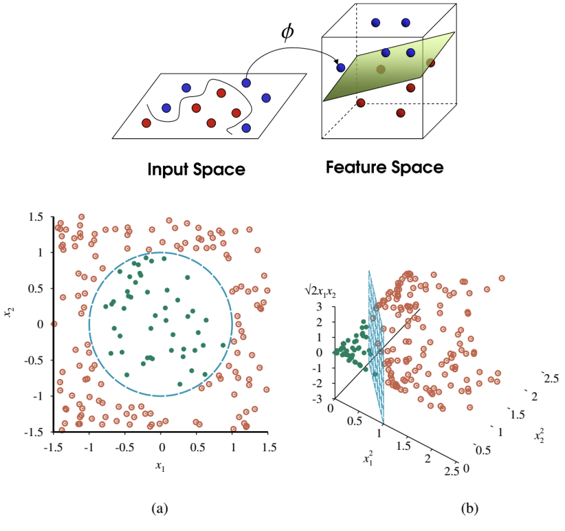
2. SVM은 linear separating hyperplane을 생성하지만, kernel trick을 사용해 데이터를 더 높은 차원의 공간으로 embedding 할 수 있음. 원본 input space에서 linearly separable 하지 않은 데이터가 고차원 공간에서는 쉽게 분리되는 경우가 많음
3. SVM은 nonparametric임. Separating hyperplane은 parameter 값의 집합이 아닌 example point 집합에 의해 정의됨. Nearest-neighbor model은 모든 example을 유지해야 하지만, SVM model은 separating plane에 가장 가까운 example (일반적으로 차원 수의 몇 배에 불과한)만 유지. 따라서 SVM은 nonparametric model과 parametric model의 장점을 결합: 복잡한 함수를 표현하는 유연성을 가지면서 overfitting에 강함

Properties of SVMs

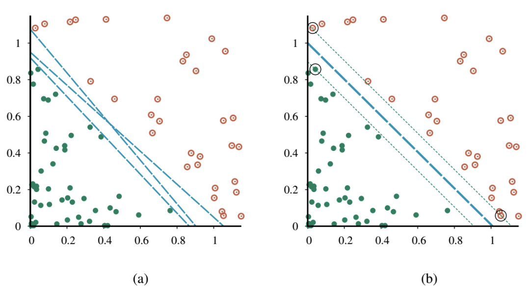
SVM은 maximum margin separator를 구축
Margin은 그림의 점선으로 둘러싸인 영역의 너비 (separator에서 가장 가까운 example point까지 거리의 2배)
SVM은 데이터를 더 높은 차원의 공간으로 embedding 하는 능력(kernel trick)을 가짐
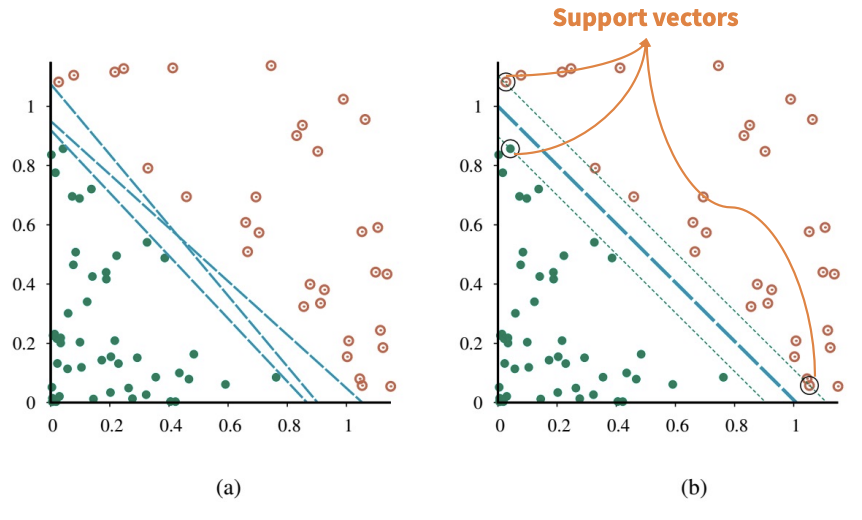
SVM은 nonparametric임. Separating hyperplane은 parameter 값의 집합이 아닌 example point 집합에 의해 정의됨
Logistic regression은 어떤 separating line을 찾으며, 이 line의 정확한 위치는 모든 example point에 따라 달라짐
SVM의 핵심 통찰은 일부 example (즉, support vector)이 다른 것보다 더 중요하며, 이에 집중하는 것이 더 나은 generalization으로 이어질 수 있다는 것

Implementing ML Models in Python

Scikit-learn

https://scikit-learn.org/

K-NNs in Scikit-learn

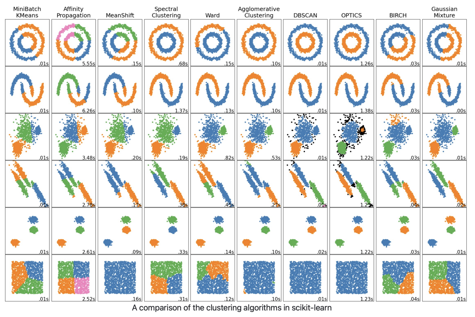
https://scikit-learn.org/stable/auto_examples/neighbors/plot_classification.html#sphx-glr-autoexamples-neighbors-plot-classification-py

Clustering in Scikit-learn

alt text

(Gaussian) Naïve Bayes in Scikit-learn

https://scikit-learn.org/stable/modules/naive_bayes.html

GaussianNB는 classification을 위한 Gaussian Naive Bayes algorithm을 구현함. Feature의 likelihood는 Gaussian이라고 가정:

P(x_i | y) = \frac{1}{\sqrt{2\pi\sigma^2_y}}\exp\left(-\frac{(x_i - \mu_y)^2}{2\sigma^2_y}\right)

Parameter $\sigma_y$ 와 $\mu_y$ 는 maximum likelihood를 사용하여 추정

>>> from sklearn.datasets import load_iris
>>> from sklearn.model_selection import train_test_split
>>> from sklearn.naive_bayes import GaussianNB
>>> X, y = load_iris(return_X_y=True)
>>> X_train, X_test, y_train, y_test = train_test_split(X, y, test_size=0.5, random_state=0)
>>> gnb = GaussianNB()
>>> y_pred = gnb.fit(X_train, y_train).predict(X_test)
>>> print("Number of mislabeled points out of a total %d points : %d"
...       % (X_test.shape[0], (y_test != y_pred).sum()))
Number of mislabeled points out of a total 75 points : 4

Decision Trees in Scikit-learn

https://scikit-learn.org/stable/auto_examples/tree/plot_iris_dtc.html

SVMs in Scikit-learn

https://scikit-learn.org/stable/auto_examples/svm/plot_separating_hyperplane.html#sphx-glrauto-examples-svm-plot-separating-hyperplane-py

Neural Networks and Deep Learning (1)

Introduction to Neural Networks and Deep Learning

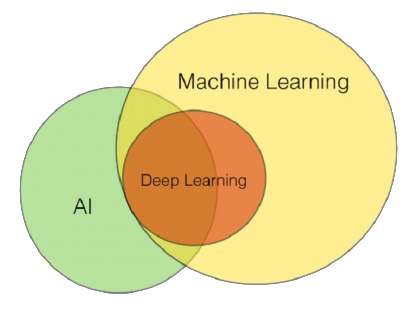
AI, ML, and DL (The Slide From the First Lecture)

Artificial Intelligence (AI), Machine Learning (ML), Deep Learning (DL)
이 용어들은 미디어와 대중이 별다른 주의 없이 상호 교환적으로 활용하는 경우가 많음
2010년대 statistical machine learning의 전례 없는 성공은 AI의 다른 모든 접근 방식을 압도했으며, 일부 (특히 비즈니스계)에서는 "artificial intelligence"라는 용어를 "neural network를 사용한 machine learning"을 의미하는 데 사용
AI, ML, DL의 계층 구조
ML은 보통 AI의 부분집합으로 간주되며, DL은 ML의 특정 부분
그러나 ML이 전적으로 AI에 포함되는지에 대해서는 여전히 논란이 있음

Deep Learning

Deep learning은 machine learning을 위한 광범위한 technique family이며, hypothesis는 조정 가능한 연결 강도를 가진 복잡한 대수적 circuit 형태를 띰
"Deep"이라는 단어는 circuit이 일반적으로 많은 layer로 구성되어 input에서 output까지의 계산 경로가 여러 단계를 거친다는 사실을 의미
Deep learning은 현재 visual object recognition, machine translation, speech recognition, speech synthesis, image synthesis와 같은 application에 가장 널리 사용되는 접근 방식
Computer Vision
Natural Language Processing
Speech & Music Processing
Reinforcement Learning
Healthcare, Legal, …
Physical AI & Robotics

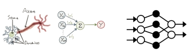
Neural Networks

Deep learning은 뇌의 neuron network를 computational circuit으로 modeling 하려던 초기 연구에 기원을 둠
이러한 이유로 deep learning method로 훈련된 network는 종종 neural network라고 불림 (실제 neural cell 및 구조와의 유사성은 피상적일지라도)

Why is Deep Learning Successful?

Deep learning 성공의 진정한 이유는 아직 완전히 밝혀지지 않았지만, 다른 method에 비해 명백한 이점을 가짐
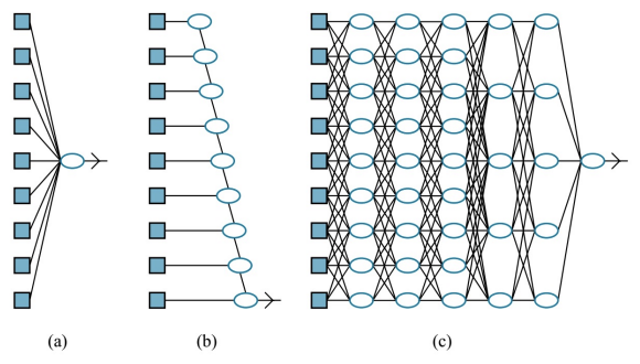
Linear/logistic regression은 많은 input 변수를 처리할 수 있지만, 각 input에서 output까지의 계산 경로는 매우 짧음 (단일 weight와의 곱셈 후 aggregate output에 더해짐)
더욱이, 서로 다른 input 변수들은 서로 상호작용 없이 ( (a) ) output에 독립적으로 기여. 이는 해당 model의 expressive power를 현저히 제한
대부분의 실제 real-world concept은 훨씬 더 복잡하지만, 이 model들은 input space에서 linear function과 경계만 표현 가능
Decision tree는 많은 input 변수에 의존할 수 있는 긴 계산 경로를 허용
그러나 이는 가능한 input vector 중 상대적으로 작은 부분에 대해서만 해당 ( (b) ). Decision tree가 가능한 input의 상당 부분에 대해 긴 계산 경로를 가진다면, input 변수의 수에 대해 exponentially large 해야 함
Deep learning의 기본 아이디어는 계산 경로가 길도록 circuit을 훈련하는 것
모든 input 변수가 복잡한 방식으로 상호작용하도록 허용 ( (c) )
이러한 circuit model은 많은 중요한 learning problem 유형에 대해 real-world data의 복잡성을 포착할 만큼 충분히 expressive 한 것으로 밝혀짐

Simple Feedforward Networks

Feedforward Networks

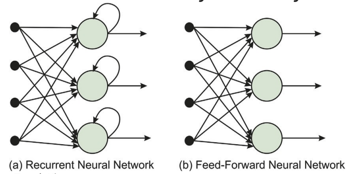
(Deep) feedforward (neural) network (또는 multi-layer perceptrons (MLPs))는 한 방향으로만 connection을 가짐
지정된 input 및 output node가 있는 directed acyclic graph를 형성
각 node는 input의 함수를 계산하고 그 결과를 network의 후속 node로 전달
정보는 input node에서 output node로 network를 통해 흐르며, loop가 없음
Recurrent network는 중간 또는 최종 output을 자체 input으로 다시 feedback
이는 network 내의 signal 값이 internal state 또는 memory를 갖는 dynamical system을 형성함을 의미
Neural network에서 input 값은 일반적으로 continuous하며, node는 continuous input을 받아 continuous output을 생성
Node에 대한 input 중 일부는 network의 parameter
Network는 이 parameter 값을 조정하여 network 전체가 training data에 맞도록 학습
Feedforward network의 목표는 어떤 함수 $f^*$ 를 근사(approximate)하는 것
예: Classifier의 경우 $y = f^*(\mathbf{x})$ 는 input $\mathbf{x}$ 를 category $y$ 로 mapping
Feedforward network는 $y = f(\mathbf{x};~ \boldsymbol{\theta})$ 라는 mapping을 정의하고, 최상의 함수 근사(approximation)를 결과로 내는 parameter $\boldsymbol{\theta}$ 의 값을 학습
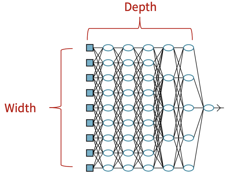
Feedforward network는 일반적으로 많은 서로 다른 함수를 함께 구성(composing)하여 표현되기 때문에 network라고 불림
예: $f^{(1)}$ , $f^{(2)}$ , $f^{(3)}$ 세 함수가 chain으로 연결되어 $f(\mathbf{x}) = f^{(3)}(f^{(2)}(f^{(1)}(\mathbf{x})))$ 를 형성
이 경우 $f^{(1)}$ 은 network의 첫 번째 layer, $f^{(2)}$ 는 두 번째 layer라고 불림
Chain의 전체 길이가 model의 depth를 결정. "Deep learning"이라는 이름이 여기서 유래
Feedforward network의 마지막 layer는 output layer라고 불림
Input layer와 output layer 사이의 layer들은 hidden layer라고 불림
- Network의 각 hidden layer는 일반적으로 vector-valued
- 이러한 hidden layer의 dimensionality가 model의 width를 결정
Vector의 각 element는 neuron과 유사한 역할을 하는 것으로 해석될 수 있음
또한 layer가 병렬로 작동하는 많은 unit으로 구성되어 있으며, 각 unit은 vector-to-scalar 함수를 나타낸다고 생각할 수 있음
각 unit은 많은 다른 unit으로부터 input을 받고 자신의 activation value를 계산한다는 의미에서 neuron과 유사
그러나 neural network의 목표는 뇌를 완벽하게 model 하는 것이 아님

Computation of Feedforward Networks

Network 내의 각 node를 unit (또는 perceptron)이라고 함
- 전통적으로 unit은 (1) 이전 node들로부터의 input의 weighted sum을 계산하고 (2) nonlinear function을 적용하여 output을 생성
- $a_j$ 를 output unit $j$ 라 하고 $w_{i,j}$ 를 unit $i$ 에서 unit $j$ 로의 link에 연결된 weight라 할 때;
$a_j = g_j(\sum_i w_{i,j} a_i) \equiv g_j(in_j)$
- 여기서 $g_j$ 는 unit $j$ 와 연관된 nonlinear activation function이고, $in_j$ 는 unit $j$ 로의 input의 weighted sum
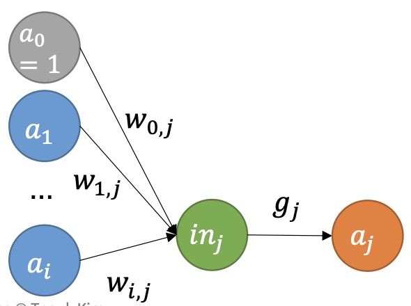
- 앞의 방정식을 vector 형태로 작성 가능
$\mathbf{a} = \mathbf{g}(\mathbf{W}\mathbf{x})$
Activation function이 nonlinear라는 사실이 중요
- 만약 그렇지 않다면, unit의 모든 구성(composition)은 여전히 linear function을 나타낼 것 ( $W = W_1W_2$ 일 때 $\mathbf{W}\mathbf{x} = \mathbf{W_1}\mathbf{W_2}\mathbf{x}$ )
- Nonlinearity는 충분히 큰 unit network가 임의의 함수를 표현할 수 있게 하는 요소
Universal approximation theorem
- Computational unit의 layer가 두 개뿐인 network (첫 번째는 nonlinear, 두 번째는 linear)가 임의의 continuous function을 임의의 정확도로 근사(approximate)할 수 있음을 명시

Activation Funtions

다양하고 서로 다른 activation function이 사용됨
Logistic 또는 sigmoid function (logistic regression에서도 사용):

\sigma(x) = 1/(1 + e^{-x})

ReLU function (Rectified Linear Unit의 약어):

\text{ReLU}(x) = \max(0,~x)

Softplus function (ReLU function의 smooth version)
Tanh function:

\tanh(x) = \frac{e^{2x} - 1}{e^{2x} + 1}